A New View of Statistics	© 1997 Will G Hopkins
Go to: Next · Previous · Contents · Search · Home

Generalizing to a Population:
SAMPLE SIZE ON THE FLY continued

 ON THE FLY FOR DIFFERENCES BETWEEN MEANS

A variant of the method also works for longitudinal studies--for example, where you want to compare the strength of females before and after they take a hormone that makes them like males. We'll come to those in a minute.
 
 Cross-Sectional Studies

Recall that the effect size is the difference between the means divided by the average standard deviation of the two groups. Well, the standard deviation calculated from your sample introduces some error of its own, which contributes to error in the effect size. So if you have a more accurate estimate of the population standard deviation from elsewhere, use it instead of the value from your sample. It can mean 40 less subjects, depending on how big the effect is. It also makes calculating the confidence limits of the effect size a lot easier.

Here's the method, for either standard deviation.

1. Start with about 40 or more subjects (20 or more in each group), knowing that you might have to go to nearly 400 if the effect turns out to be trivial.
2. If validity is less than perfect, inflate the starting number and make further adjustments as described for correlations. Not an easy task!
3. Do the practical work, then calculate the difference between the means.
4. Convert the difference between the means into an effect size by dividing it by the standard deviation. Use the population standard deviation if available, or calculate the average standard deviation of your two groups if not. Make sure you average the variances of the two groups, then take the square root to get the average standard deviation. Don't forget to log or rank transform the dependent variable if necessary (which may complicate the use of any available population standard deviation).
5. Use the appropriate curve on this graph to read off the sample size needed to give an acceptable confidence interval to your effect size. Or license holders can use the spreadsheet, which also adjusts for validity.
   

   Each curve was drawn through the point in the middle of each step of the scale that gives a confidence interval just spanning the step. See the simulation program for more information.

6. If the sample size from the graph is less than the initial sample size, the confidence interval is already narrower than the acceptable confidence interval, so the study is finished. Otherwise go to the next step.
7. Subtract the current total sample size from that sample size on the graph. The result is the number of subjects for the next lot of practical work. You can "cheat" by doing the practical work on less than this number, if it's a big leap to nearly 400 from the previous number. This trick will help make sure you don't test too many subjects, as I described for correlations. If the effect turns out to be trivial, you will still eventually end up with nearly 400, of course!
8. Divide the extra subjects equally into the two groups, do the practical work, add the new observations to all the previous ones, then calculate the effect size for the whole lot.
9. If the effect size is greater than the previous value, the confidence interval must be narrower than the acceptable confidence interval, so the study is finished. Otherwise go to the next step.
10. Use the graph to read off the sample size needed to give an acceptable confidence interval to your effect size. Now go to Step 7, and continue in this fashion until you reach a sample size that gives an acceptable confidence interval.

Cool! You've got a value for the effect size, and you've done it with the minimum number of subjects, and it's practically unbiased by doing it on the fly, and you know that its confidence interval is narrow enough that it can't overlap more than two steps (colors) on the qualitative magnitude scale. But what exactly is the value of the confidence interval? If I end up refereeing your paper, I'll insist you put it in! Here's how to get it.
 
Confidence Limits for Effect Size (Cross-sectional Studies)
 
If you used the population standard deviation for sample sizing on the fly, get your stats program to produce the confidence interval of the raw difference between the means for the final sample. Divide this confidence interval by the population standard deviation and you have the exact confidence interval for the effect size. The observed effect size sits symmetrically in the middle of this confidence interval. If you can't get your stats program to produce the confidence interval of the difference score, the confidence interval of the effect size is given exactly by 2t·sqrt(4/N), where N is the total sample size, and t is the value of the t statistic for N - 2 degrees of freedom and cumulative probability 0.975. The value of t is near enough to 2.0.

If you used the sample standard deviation on the fly, the resulting effect size is biased a bit high for small total sample sizes (N). Adjust out the bias using this formula:
          unbiased ES = (observed ES)(1 - 3/(4N - 1)).
Now use the following fairly accurate formula to calculate the 95% confidence interval for the unbiased effect size:
          95% confidence interval = 4sqrt(4/N + ES²/(N - 2)).
The confidence limits are therefore given fairly accurately by:
          ES ± 2sqrt(4/N + ES²/(N - 2)),
but that's only for ES<1.0. For larger values of ES, the limits start to sit asymmetrically about the observed value of ES. Then the going gets really tough. The exact values of the confidence limits are given by t·sqrt(4/N), where t is the value of the non-central t statistic with degrees of freedom = N - 2, non-central parameter = ES·sqrt(N/4), and cumulative probabilities of 0.025 and 0.975 for the lower and upper limits respectively. Only advanced stats programs can produce values for the non-central t statistic.

All the above formulae are available on the spreadsheet, with the exception of the non-central t statistic. I will add it when Excel does.

Reference for formulae:
Becker, B. J. (1988). Synthesizing standardized mean-change measures. British Journal of Mathematical and Statistical Psychology, 41, 257-278.
 
 Longitudinal Studies

But if we use the sample standard deviation to calculate the effect size, there is a major hitch. With the small sample sizes that are possible, the error in the standard deviation is proportionally larger, so the confidence interval of the effect size ends up large after all, so we lose the benefit of the high reliability and end up with larger sample sizes again. The calculations are difficult, too.

On the other hand, if we know or can guess the population standard deviation, all is saved. So I'll concentrate on a method that uses the population standard deviation, then deal briefly with the use of the sample standard deviation.
 
Using Population SD to Calculate Effect Size and its Confidence Limits
 
This method works for the effect size in cross-sectional or longitudinal designs of any kind, and for any estimates/contrasts between levels of within and between factors. Wow! The only challenge for you is to coax your stats program to produce a confidence interval for the raw difference between the means, or for whatever estimate/contrast you are interested in. You then simply convert that to a confidence interval for the effect size by dividing it by the population standard deviation, see if the confidence interval is narrow enough, and if it's not, work out how many more subjects you'll need.

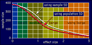
This paragraph may confuse you. Skip to the method in the next paragraph if it does. To get an idea of the kind of sample sizes you can end up with, you can apply the formulae I presented earlier for the effects of reliability on sample size. The only difference is, the "N" in the formulae is now the sample size you would need for a cross-sectional study, as shown by the curve in the above graph for population SD. So, the sample size for a longitudinal study with a single pre and post measurement and no control group is N(1 - r)/2, where r is the reliability correlation coefficient. If there is a control group, you need twice as many in both groups, or 2N(1 - r) altogether. Let's check out an example on the graph above. If your effect size turns out to be in the middle of the medium range, you'd end up needing about 200 subjects for a cross-sectional study. But if your reliability is 0.9, that'll come down to 10 subjects for a study without a control group! Fantastic! If your reliability is 0.95--not out of the question for some outcome measures--you'd need only 10 subjects in each group of a properly controlled study. It will be even less for larger effects. But check the graph: you might still have to go to nearly double that number if the effect size turns out to be zero.

OK, here's how the method works. It's the usual iterative process, but this time it relies on the fact that the width of the confidence interval is inversely proportional to the square root of the sample size.

1. If you have high reliability and the effect is very large, ridiculously small sample sizes are possible. But you have to be careful when you're down to five or so subjects, because you might end up with a sample that is not typical of the population. Papers do get published with six subjects in each group, but I'd feel safer with a minimum of eight. If your reliability is unlikely to be better than 0.9, or your effects are probably small-medium, start with 10-15. That means 10-15 in a single group if it's a study without a control group, or 10-15 in each group if there's a control group or several experimental groups.
2. Do the practical work, then crunch the numbers to get the difference between the means of interest, or do whatever other estimate/contrast you like. By the way, when you have a control group, the difference you want is the post-pre difference score for the experimental group minus the post-pre difference score for the control group.
3. Get your stats program to produce the confidence interval for the difference. Convert it into effect-size units by dividing it by the population standard deviation. Convert the difference itself into an effect size in the same way.
4. Use this figure to read off the acceptable confidence interval for your effect size, or use the spreadsheet, which also performs subsequent calculations and takes account of less-than-perfect validity.
   

   The way I derived this curve and validated the on-the-fly method is described on separate pages for longitudinal studies without a control group and with a control group.

5. If your observed confidence interval is less than the acceptable confidence interval, the study is obviously finished. If not, go to the next step.
6. Divide your observed confidence interval by the acceptable confidence interval, square the result, then multiply it by the total number of subjects you have tested. That's your next target total number of subjects.
7. Subtract the current total sample size from that target total. The result is the extra subjects for the next lot of practical work. Divide them equally into the groups, if there is more than one group.
8. Do the practical work, add the data to the previous data, then go to Step 3.

The confidence interval of the final effect size is no problem, this time. You've been calculating it all along.
 
Using Sample SD to Calculate Effect Size and its Confidence Limits
 
You go through the same steps as for use of the population SD, but you have to calculate the confidence interval for the effect size using the sample SD. You then use this calculated confidence interval in Step 3. Here's how to calculate the confidence interval. If you have a control group, I will assume it has the same number of subjects as the experimental group.

• Calculate the effect size using the average variance, as described in Step 4 for cross-sectional studies. If you've got a control group too, average all four variances before you take the square root.
• Correct out the bias in the effect size, using this formula:
  unbiased ES = (observed ES)(1 - 3/(4N - 1)), where N is the total sample size (experimental plus any control).
• Calculate the reliability (r) of the dependent variable, preferably as an intraclass correlation, but otherwise as a Pearson correlation. Do it using the experimental data: a shift in the mean due to the intervention does not affect the reliability. If you have a control group, use the average reliability of the control and experimental group. A proper average should be done via the Fisher z transform, but if the correlations are fairly similar it won't matter if you just take the usual mean.
• Calculate an approximate confidence interval for the ES using this formula:
  4sqrt(2(1 - r)/N + ES²/(2(N - 1)) if there is no control group, or
  4sqrt(8(1 - r)/N + ES²/(2(N - 4)) if there is a control group.

When you've done your sampling on the fly, the confidence limits of the effect size, for effect sizes <1, are given by the final effect size ± half the confidence interval. For effect sizes>1 there is that problem of the confidence interval not sitting symmetrically around the effect size...

For studies without a control group, the exact values of the confidence limits are given by t·sqrt(4(1 - r)/N), where t is the value of the non-central t statistic with degrees of freedom = N - 2, non-central parameter = ES·sqrt(N/(4(1 - r)), and cumulative probabilities of 0.025 and 0.975 for the lower and upper limits respectively.

For studies with a control group, the exact values of the confidence limits are given by t·sqrt(8(1 - r)/N), where t is the value of the non-central t statistic with degrees of freedom = N - 2, non-central parameter = ES·sqrt(N/(8(1 - r)), and cumulative probabilities of 0.025 and 0.975 for the lower and upper limits respectively.

If only the stats programs would do these calculations...! I've put most of them on the spreadsheet, but I can't do anything about non-central t statistics until Excel does.

If you've got this far, you will no doubt be interested in a simulation that validates the on-the-fly method for the case of no control group. It includes an empirical check on the formulae when there is a control group.

Now for something a little easier: on the fly for differences in frequencies.