GENERALIZING
TO A POPULATION
You have a bunch of numbers for a
sample of subjects. But people don't really want to know about
your sample, which was a one-off set of observations that will never
be taken again. People are much more interested in what you can say
about the population from which your sample was drawn. Why?
Because things that are true for the population are true for a lot
more people than just for your sample. Hence the second major purpose
of statistics: generalizing from a sample to a population.
It's also known as making inferences about a population on the
basis of a sample. By the way, the term population doesn't
mean the entire population of a country. It just means everyone in a
well-defined group; for example, young adult male trained distance
runners.
I deal first with confidence limits, which are the simplest and best
way to understand generalization. Bootstrapping, meta-analysis,
and Bayesian analysis are applications of confidence limits that I include
on this page. On the next page are the related concepts
of p values and statistical significance, followed
by type I and II errors and a mention of bias. You can also
download a slideshow that deals with all the
material on these three pages, and more.
The second section is devoted to how we use statistical
models or tests to generalize the relationships between variables.
To generalize properly you need a sample of adequate size, so I deal with methods
for estimating sample size in the final section.
Generalizing
to a Population: CONFIDENCE LIMITS
 GENERALIZING
VIA CONFIDENCE LIMITS
What can you say about the
population when all you've got is a sample? Well, to start with, the
value of a statistic (e.g. a correlation coefficient) derived from a
sample is obviously one estimate of the value in the population. But
the sample is only an approximation for the population, so the
statistic is also only an approximation. If you drew a different
sample, you'd get a different value.
The only way you can really get the population value is to measure
everyone in the population. Even if that was possible, it would be a
waste of resources. But it is possible to use your sample to
calculate a range within which the population value is likely to
fall. "Likely" is usually taken to be "95% of the time," and the
range is called the 95% confidence interval. The values at
each end of the interval are called the confidence limits. All
the values between the confidence limits make up the confidence
interval. You can use interval and limits almost
interchangeably.
Learn this plain-language definition: the confidence interval is the likely
range of the true value. Note that there is only one true value,
and that the confidence interval defines the range where it's most likely to
be. The confidence interval is NOT the variability of the true value or of any
other value between subjects. It is nothing like a standard deviation. If there
are individual differences in the outcome,
then there is more than one true value, but we'll deal with that later.
Another important concept embodied in confidence limits is precision of
estimation. The wider the confidence interval, the less the precision. Research
is all about getting adequate precision for things like a correlation
coefficient, a difference in the mean between groups, the change in a mean following
a treatment, and so on.
 An
Example
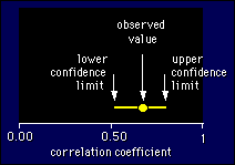
Suppose you observed a correlation of 0.68
between height and weight of 64 healthy undergraduate females. The
95% confidence limits are 0.52 and 0.79, which means that there's a
95% chance that the correlation between more-or-less all
healthy undergraduate females is between 0.52 and 0.79. The figure
shows it graphically. The confidence interval is the length of the
line between the limits. You would report this result formally in a
research paper as follows: the correlation between height and weight
was 0.68; the 95% confidence interval was 0.52 to 0.79. I prefer the
following less formal rendition: the correlation... was 0.68, and the
likely range was 0.52 to 0.79.
Notice that the confidence limits in the above example are not
spaced equally on each side of the observed value. That happens with
non-normally distributed statistics like the correlation coefficient.
Most other statistics are normally distributed, so the observed value
falls in the middle of the confidence interval. For example, an
observed enhancement in performance of 2.3% could have confidence
limits of 1.3 to 3.3%. In such cases, you can use a ± sign to
express the outcome in the following way: the enhancement was 2.3%,
and the likely range (or confidence interval or limits) was
±1.0%. Of course, you mean by this that the limits are 2.3-1.0
and 2.3+1.0.
The lower and upper confidence limits need to be interpreted
separately. The lower (or numerically smaller) limit shows how
small the effect might be in the population; the upper
limit shows how large the effect might be. Of course, you'll never
know whether it really is that small or big unless you go out and
measure the whole population. Or more subjects, anyway. Which brings
us to the next important point: the more subjects, the narrower the
confidence interval.
 Effect
of Sample Size on the Confidence Interval
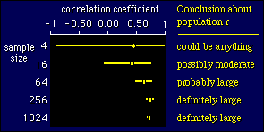
Here's a figure showing how the
width of the confidence interval depends on the number of subjects,
for a correlation coefficient. It's the sort of thing you would get
if you took bigger and bigger samples from a population.

Notice that you can't say anything useful about the population correlation
when the sample has only 4 subjects. Already with 16 subjects you get the idea
that it could be moderately positive. With 64 subjects the correlation is definitely
positive and probably large, although it could also be moderate. The sample
of 256 nails it as a large effect, and 1024 subjects give too much precision.
The conclusions I have shown in the above figure are only approximate. Since
drawing this figure, I have come up with an exact approach to making conclusions
like probably large. See below.
 The
Confidence Interval and Statistical Significance
If the confidence interval does not
overlap zero, the effect is said to be statistically
significant. In the above figure, the results for the sample
sizes of 64, 256, and 1024 are all statistically significant, whereas
the other results are not statistically significant. We can also
define statistical significance using something called a p
value, but I'll deal with that on the next page.
We have a couple of plain-language ways of talking about something
that is statistically significant: we say that the true value is
unlikely to be zero, or that there is a real effect. These
aren't bad ways to think about statistical significance, and you can
sort of understand them by looking at the above figure, but they're
not strictly correct. After all, the true value of something is never
exactly zero anyway. I'll pick this issue up on the next page, under
hypothesis testing.
The value for a statistic corresponding to no effect in the
population is called the null value. For correlations and
changes in the mean, the null value is zero. If the outcome statistic
is a relative risk or odds ratio, the null value is 1 (equal risk or
odds). So for these statistics, the result is statistically
significant if the confidence interval does not overlap 1.
 A
Spreadsheet for Confidence Limits
To calculate confidence limits for a statistic,
a stats program works out the variation between subjects, then estimates how that
variation would translate into variation in your statistic, if you kept taking
samples and measuring the statistic. (You don't have to take extra samples to
get the variation from sample to sample.) When you tack that variation onto the
value of your sample statistic, you end up with the confidence interval. The calculation
requires some important simplifying assumptions, which I will deal with later.
Unfortunately, some stats programs don't provide confidence limits, but they
all provide p values. I've therefore made a spreadsheet to calculate confidence
limits from a p value, as explained on the next
page. The calculation works for any normally distributed outcome statistic,
such as the difference between means of two groups or two treatments. I've included
calculations for confidence limits of relative risks and odds ratios, correlations,
standard deviations, and comparison (ratio) of standard deviations.
I've also added columns to give chances of clinically
or practically important effects. Make sure you come to terms with this
stuff. It is more important than p values.
Update Oct 2007: the spreadsheet now generates customizable
clinical and mechanistic inferences, consistent with an article
on inferences in Sportscience in 2005. The inferences are also consistent
with an article on sample-size
estimation in Sportscience in 2006.
| Spreadsheet for confidence limits and inferences:
Download |
 Bootstrapping
(Resampling)
Another way of getting confidence limits, when
you have a reasonable sample size, is by the wonderful new technique of bootstrapping.
It's a way of calculating confidence intervals for virtually any outcome statistic.
It's tricky to set up, so you use it only for difficult statistics like the difference
between two correlation coefficients for the same subjects. And you'll need an
expert with a high-powered stats program to help you do it.
For example, you might want to use a fitness test in a large study, so you
do a pilot first to see which of two tests is better. The tests might be submaximal
exercise tests to determine maximum oxygen uptake. "Better" would mean the test
with higher validity, in other words the test with the higher correlation with
true maximum oxygen uptake. So you might get a sample of 20 subjects to do the
two tests and a third maximal test for true maximum oxygen uptake. The validity
correlations turn out to be 0.71 and 0.77. Sure, use the test with the higher
correlation, but what if it's more difficult to administer? Now you begin to
wonder if the tests are really that different. The difference is 0.06.
That's actually a trivial difference, and if it was the real difference, it
wouldn't matter which test you used. But the observed difference is never the
real difference, and that's why we need confidence intervals. If the confidence
interval was 0.03 to 0.09, you'd be satisfied that one test is a bit better
than another, but that it still doesn't really matter, and you would choose
the easier test. If the confidence interval was -0.11 to 0.23, you couldn't
be confident about which test is better. The best decision then would be to
test more subjects to narrow down the confidence interval.
Anyway, bootstrapping is how you can get the confidence interval.
The term bootstrapping refers to the old story about people
lifting themselves off the ground by pulling on the backs of their
own boots. A similar seemingly impossible thing occurs when you
resample (to describe it more formally) to get confidence
intervals. Here's how it works.
For a reasonably representative sample of maybe 20 or more
subjects, you can recreate (bootstrap) the population by duplicating
the sample endlessly. Sounds immoral, if not impossible, but
simulations have shown that it works! Next step is to draw, say, 1000
samples from this population, each of the same size as your original
sample. In any given sample, some subjects will appear twice or more,
while others won't be there at all. No matter. Next you calculate the
values of the outcome statistic for each of these samples. In our
example above, that would be the difference between the correlations.
Finally, you find the middle 95% of the values (i.e. the 2.5th
percentile and the 97.5th percentile). That's the 95% confidence
interval for your outcome! Cool, eh?
The median value from your 1000 samples should be virtually the same
as the value from the original sample. If it's not, something is
wrong. Sometimes the variables have to be transformed in some
way to get over this problem. For example, to get the confidence
interval for the difference between correlation coefficients, you
first have to convert the correlations using something called the
Fisher z transformation:
z = 0.5log[(1 + r)/(1 - r)].
This equation looks horribly complicated, but all it does is make the
correlations extend out beyond the value 1.0. It makes them behave
like normally distributed variables.
How do you "duplicate endlessly" to recreate the population?
Actually you don't duplicate the data set. If your original sample
had 20 observations, you use a random number generator in the stats
program to select a sample of 20 from these 20. Then you do it again,
and again, and again...
At the moment I don't know of a good rule to decide when a sample
is big enough to use bootstrapping. Twenty observations seems to be
OK. Note, though, that if you have subgroups in your data set that
are part of the outcome statistic, you need at least 20 in each
subgroup. For example, if you wanted to compare a correlation in boys
and girls, you would need at least 20 boys and 20 girls.
And now for a test of your understanding. If you can recreate the
population by duplicating the sample endlessly, why bother with all
that resampling stuff? Why not just work out the value of the
statistic you want from say a one-off sample of a million
observations taken from this population? With a million observations,
it will be really accurate! Answer: Well, ummm... the value you
calculate from a million observations will be almost exactly the same
as the value from your original sample of 20. You're no better off.
OK, it was a silly question.
 Meta-Analysis
I deal with meta-analysis here,
because it is an application of confidence intervals. Meta-analysis
is literally an analysis of analyses, which is near enough to what it
is really: a synthesis of all published research on a particular
effect (e.g. the effect of exercise on depression). The aim is to
reach a conclusion about the magnitude of the effect in the
population.
The finding in a meta-analytic study is the mean effect of all the
studies, with an overall confidence interval. In deriving the mean,
more weight is given to studies with better designs: more subjects,
proper random selection from the population, proper randomization to
any experimental and control groups, double blinding, and low dropout
rate. Studies that don't meet enough criteria are sometimes excluded
outright from the meta-analysis.
Whenever you read a meta-analysis involving longitudinal
(experimental) studies, check to make sure the statistician used the
correct standard deviation to calculate the effect size. It should
always be the average standard deviation of the before and/or after
scores. Some statisticians have used the standard deviation of the
before-after difference score, which can make the effects look much
bigger than they really are.
 Bayesian
Analysis
Bayesian analysis is a kind of
meta-analysis in which you combine observed data with
your prior belief about something and end up with a
posterior belief. In short, it's a way to update your
belief. Clinicians use this approach informally when they try to
diagnose a patient's problem. They have a belief about possible
causes of the problem, and they probe for symptoms, test for signs of
possible diseases, and order blood tests or scans or whatever to get
data that will make their belief in one cause much greater than other
possible causes. Fine, and no-one disputes the utility of this
approach in the clinical setting with an individual patient or
client. The disputes arise when statisticians try to apply it to the
analysis of research data from a sample of a population. Let's start
with the usual approach (also known as the frequentist
approach) to such data, then see how a Bayesian would handle it.
Suppose you're interested in the effect of a certain drug on performance. You
study this problem by conducting a randomized controlled trial on a sample of
a population. You end up with confidence limits for the true effect of the drug
in the population. If you're a frequentist you publish the confidence limits.
But if you're a Bayesian, you also factor in your prior belief about the efficacy
of the drug, and you publish credibility limits representing your posterior
(updated) belief. For example, you might have believed the drug had no effect
(0.0%), and you were really skeptical, so you gave this effect confidence limits
of -0.5% to +0.5%. You then did the study and found a positive effect of 3.0%,
with confidence limits of 1.0% to 5.0%. Combine those with your prior belief
and you end up with a posterior belief that the effect of the drug is 0.6%,
with confidence limits of -1.0% to 3.2%. Let's assume a marginal effect is 1%,
a small effect is 3%, and a moderate effect is 5%. A Bayesian concludes (from
the credibility limits of -1.0% to 3.2%) that the drug has anything from a marginal
negative effect to a small positive effect. A frequentist concludes (from the
confidence limits of 1.0% to 5.0%) that the drug has anything from a marginal
positive to a moderate positive effect.
There are formal procedures for combining your prior belief with
your data to get your posterior belief. In fact, the procedure works
just like a meta-analysis of two studies: the first study is the one
you've just done to get an observed effect with real data; the other
"study" is your prior belief about what the effect was. The observed
effect and your belief are combined with weighting factors inversely
proportional to the square of the widths of their confidence
intervals. For example, if you have a very strong prior belief, your
confidence (= credibility) interval for your belief will be narrow,
so only a markedly different observed effect with a narrow confidence
interval will change your belief. On the other hand, if you are not
at all sure about the effect, your confidence interval for your prior
belief will be wide, so the confidence limits for your posterior
belief won't be much different from those provided by the data. To
take this example to an extreme, if you have no prior belief, the
posterior confidence limits are identical to those provided by the
data.
A positive aspect of the Bayesian approach is that it encapsulates
the manner in which we assimilate research findings. New evidence
that agrees with our preconceived notions reinforces our beliefs,
whereas we tend to disregard evidence that flies in the face of our
cherished prejudices or has no apparent mechanism. Sure, but even as
a frequentist you can tackle these issues qualitatively in the
Discussion section of your paper. If you try to quantify your
prior belief, you run into two problems. First, your belief and the
real data are combined with weighting factors, but they are otherwise
on an equal footing. That's acceptable to a frequentist only if it's
quite clear that the outcome of the Bayesian analysis is still only a
belief, not a real effect. Secondly, exactly how do you convert a
belief into a quantitative effect, and how do you give it confidence
limits? (Bayesians give their belief a complete probability
distribution, but the principle is the same.) You could--and probably
do--base the belief on the results of other studies, but you might
just as well meta-analyze these other studies to get your prior
"belief". In that case, though, your posterior "belief" will be
identical to a meta-analysis of all the studies, including the one
you've just done. In other words, it's not a Bayesian analysis any
more.
Bayesian analysis may be justified where a decision has to be made
with limited real data. The prior belief could be the average belief
of several experts. When I hear of a specific example, I will update
this page. Meanwhile, click here for a
response to this section from Mike Evans, a Bayesian.
Go to: Next
· Previous
· Contents ·
Search
· Home
Last updated 21 Oct 07

