Generalizing to
a Population:
STATISTICAL MODELS
continued
 MODELS: IMPORTANT DETAILS
On this page are details of how a stats
program fits a model, which you will need to understand before you tackle
the other major topic on this page, calculating confidence
limits and p values. You'll find that your data sometimes violate assumptions
the stats programs make when they perform the calculations. One fix--the t
test for unequal variances--is at the bottom of this page. Other fixes are
on the following pages: log transformation, rank
transformation, non-parametric models and tests,
models for ordinal dependent variables, and non-linear
models.
 How a Stats Program Fits a Model
Key terms you will meet here are parameters, predicted
values, residuals, and goodness of fit.
Parameters
Recall that, to fit a straight line to data,
you need a slope and an intercept for the line. The slope and intercept are
called parameters of the model.
If the model is a t test (for example, heights of girls vs boys) or simple
ANOVA (heights of three or more subgroups), the parameters are single values
of height for each subgroup that best fit the data. The values are, of course,
the means of each subgroup.
To complete the picture, what are the parameters if we're modeling the frequency
of something in one or more groups (for example, the prevalence of injury in
different sports)? Too easy: it's just the frequency in each group, or more
exactly, the probability that a person in a each group will have an injury or
whatever.
Solution and Residuals
As we've seen, a relationship or model is
represented by parameters like the slope and intercept of a line, or the means
of groups. To fit a model, the stats program finds values of the parameters
that fit the data best. These values are called the solution. But HOW
is it done?
The standard method is to find the values of the parameters that produce the
minimum difference between the observed values of the dependent variable
and the values of the dependent variable that would be predicted by the
model. The difference between an observed and a predicted value is a residual.
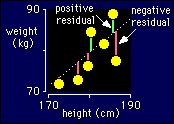 It's easiest to understand
when the model you are fitting is a straight line. See the diagram, which is
the top corner of the height-weight graph blown up so you can see what's what.
The observed values are just the weights. The predicted values are the weights
on the line corresponding to each observed weight. You should be able to see
that if you drew a straight line further away from the points, the residuals
overall would get bigger.
The program actually minimizes the sum of the squares of the residuals.
Why not just minimize the sum of the raw residuals? Let's just accept that it
works best to square the residuals first. So when you fit a straight line, it's
known as the least-squares line. This line doesn't always look quite
like the best line--the slope sometimes looks a bit too shallow--but that's
because of the way the distances are measured and minimized only in the Y direction.
Trust me, it IS the best line! The same applies when you fit curves rather than
straight lines. By the way, the root-mean-square error derived from any model
is the standard deviation of the residuals, and the mean of the residuals is
always zero.
If the model we're fitting is means for different groups (in an ANOVA), the
predicted values are just the means for each group, and the residuals are the
differences between, for example, each girl's values and the girls' mean, and
ditto the boys.. Easy stuff. And when we're looking at different frequencies
of something in different groups (contingency table), the predicted values are
just the observed frequencies. There aren't any residuals as such in that case,
but you start to get them when you have categorical modeling. No need to understand
this subtlety, though.
Goodness of Fit
I've already introduced the concept of goodness
of fit for simple linear regression. I stated that the correlation is a
good way to describe it, and that 100x the square of the correlation--the percent
of variance explained--is also used. Now that you know about residuals, I can
explain goodness of fit a bit more.
Obviously, the smaller the residuals, the better the fit. One measure of the
magnitude of the residuals is their standard deviation, alias the root mean
square error. But what can we compare the error with to get a generic measure
of goodness of fit? Answer: the standard deviation of the dependent variable
itself, before we try to fit any model. This standard deviation represents the
amount of variation in the dependent variable, and the error represents the
variation that's left over after we fit the model. But statisticians like to
make things complicated, right? So they square the standard deviation to get
total variance, and they square the error to get error variance.
The total variance minus the error variance is... wait for it... the variance
explained by the model. Divide the variance explained by the total variance
and you have something equivalent to the square of a correlation coefficient--we
call it the goodness-of-fit R2 for
the model. Multiply it by 100, and you have... the percent of total variance
explained by the model, or just the percent of variance explained. Cool!
Stats books have lots of formulae involving sums of squares, which are what
we used to use to calculate statistics in the days before computers. Sums of
squares are directly related to variances. The total sum of squares is the sum
of the squares of each observed value after the mean has been subtracted from
it. The residual sum of squares is exactly what it says. Subtract the residual
SS from the total SS, divide by the total SS, and you have another formula for
R2.
The R2 is also identical to the square of
the correlation between the observed values and the values predicted by the
model--quite a nice way of thinking about goodness of fit for a complex model.
And of course, for a simple linear regression, the R2
for the model is the same as r2, the square
of the correlation coefficient.
The stats program should give you a p value for the R2,
which will help you make decisions about the linear relationship between the
dependent variable and independent variable. What programs currently won't do
is give you confidence limits for the R2.
Maybe we don't really want it anyway. It's easier to interpret R rather than
R2, as discussed in the page on scale
of magnitudes. So take the square root of the R2,
then work out the confidence interval of this correlation using the Fisher
z transformation. (The "n" in the Fisher formula in this case is the number
of degrees of freedom for the error term in the linear model, minus 1.) I've
set it all up on the spreadsheet for
confidence limits.
Goodness of fit for models in which the dependent variable is nominal is a bit
trickier. As I mentioned earlier, goodness of fit is not usually calculated
for these models, but various analogs of the correlation coefficient (e.g. the
kappa coefficient) can be used. The clinical measures of sensitivity
and specificity can also be regarded as measures of goodness of fit.
 Calculating
Confidence Limits
Calculating the value of an effect statistic
like the difference between two means is usually easy. Calculating the confidence
interval or confidence limits and/or the p value for the true value of the statistic
is another matter. In the usual models (t tests, ANOVA, linear or curvilinear
regression), the calculations are based on three simplifying assumptions: independence
of observations, normality of sampling distribution, and uniformity
of residuals. Let's see what happens and what you have to do if your data
violate these assumptions.
Independence of Observations
Independence of observations refers to the
notion that the value of one datum is unrelated to any other datum. In other
words, knowing the value of one observation gives you no information about the
value of any other. To see what happens if this assumption is violated, let's
take an extreme case. Imagine you are doing calculations on what you think is
a large data set, but unbeknownst to you, someone has inflated the sample size
simply by duplicating every observation. The observations in such a data set
are definitely not independent! The correct confidence interval or p value for
a given effect in the data would be given by an analysis based on the original
sample size, obviously. But the confidence interval you get with the spuriously
inflated sample will be narrower (by a factor of about 1/root2, or 0.7), and
the corresponding p value will be smaller too. In general, then, lack of independence
of observations results in incorrectly narrow confidence limits and incorrectly
small p values, because the effective sample size is less than what you think
it is.
Observations that are not independent are also said to be correlated or
interdependent . There are some clever tests for independence in some specific
situations, but in general you have to decide yourself--without recourse to
statistical tests--whether there is substantial interdependence among the observations
in your data set.
An obvious example of interdependence occurs in any intervention: the subjects
each provide two or more observations before and after the intervention, and
all the observations belonging to a given subject usually have similar values
compared with values from other subjects. The usual approach to such data is
a repeated-measures analysis or mixed
modeling.
A statistic summarizing the amount of independence in
a set of observations is the degrees of freedom. Well, actually, the
degrees of freedom summarizes the amount of independence in the residuals
in your model--and that's as it should be, because the residuals are what the
stats program uses to calculate the confidence interval. The degrees of freedom
is simply the total number of independent bits of error in the residuals. Here's
an example: fit a straight line to 10 points and you will have 10 residuals
but only 8 degrees of freedom, because the model estimates two parameters--the
slope and intercept of the line. Some stats procedures account for interdependence
of residuals in some complex models by estimating a reduced number of degrees
of freedom for the residuals.
You don't have to worry about the details of degrees of freedom, but you should
be aware that the more parameters you estimate in your model, the more degrees
of freedom you lose. That's not a problem if your sample size is large, but
with a small sample size the uncertainty in the magnitude of the error will
translate into substantially wider confidence intervals, because the width of
the confidence interval is proportional to the value of a t statistic for the
number of degrees of freedom of the residuals. The effect starts to bite when
your model reduces your number of degrees of freedom to 10 or less. So if you
have small sample sizes, you'll need to keep your models simple.
Normality of Sampling
Distribution
The sampling distribution of any outcome statistic
is the distribution you would expect to get for the values of the statistic,
if you repeated your study many times. To calculate the confidence limits for
the true value of most statistics, a stats program has to assume that this distribution
is normal. If your raw data have a normal-looking distribution, the sampling
distribution of all the usual outcome statistics based on the data will definitely
be normal, so there's no problem. But even if your raw data are not normally
distributed, the sampling distribution of a given statistic is often so close
to normal that you can trust the confidence limits and p value.
Question: When can't you trust the confidence limits and p value?
Answer: Depends on how non-normal your residuals are, and how small your sample
is.
Question: How non-normal, how small, and how come!?
Answer: Let's address how come first. The residuals sort-of add together
to give you the sampling distribution of your statistic. And when you add enough
randomly varying things like residuals together, even though each of them is
not normally distributed, they smooth out into a normal distribution. You can
actually prove it mathematically, and the proof is called the central limit
theorem. Of course, the more non-normal the residuals, the bigger the sample
size you will need to get a normal sampling distribution. But there are apparently
no rules about how non-normal the residuals and how small the sample size need
to be before an analysis falls over. I could find nothing on the Web and I got
no joy when I inquired on a statistics mailing list, so I did some simulations
to find out about how non-normal and how small.
I used a variable that has grossly non-normal residuals:
an ordinal variable having only two values (0 and 1). This variable is what
researchers use to code no/yes responses or 2-point Likert scales in
questionnaires. I restricted the analyses to unpaired t tests of two groups
with various sample sizes (for example, a comparison of the responses of 10
boys vs 30 girls). I found that the confidence limits started to go wrong for
sample sizes of 10 or less if the average response in one or both groups was
<0.3 or >0.7 (corresponding to more than 70% of the responses in each
group being on one or other level of the 2-point Likert scale). I also tried
ordinal variables with 3, 4 and 5 values, corresponding to Likert scales with
3, 4 and 5 levels. For any kind of reasonably realistic spread of responses
on these scales, the confidence limits were accurate for samples of 10 or more
in each group. The confidence limits went awry only when responses were stacked
up on the bottom or top level of the scale, in the same manner as for the 2-point
scale. Even then they came right for samples of 50 or so.
My conclusion is that people (me included) have worried needlessly about non-normality
of residuals. The time to get worried is when the residuals look really awful
and you have a sample of only 10 or so subjects. When that happens, you'll have
to try other approaches: logistic regression in
the case of Likert-type responses stacked up on one or other extreme value,
and some kind of transformation for everything else. I explain transformations
on the next few pages, starting with log transformation.
By the way, do not test for non-normality of the residuals.
Residuals that look only remotely normal will work fine in your analyses, even
though the test tells you they aren't normal. And with large sample sizes, residuals
that look indistinguishable from normal sometimes return a positive test for
non-normality, but your analyses will definitely be OK here.
Uniformity
of Residuals
Your residuals are uniform if their mean is
zero and their scatter (standard deviation) is the same for any subsample or
subgroup of observations. So what does all that mean? I'll try to make
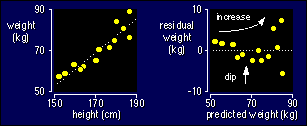
things clear with an example. Here are the data for weight vs height for the
linear regression you saw earlier. I've also plotted the residuals against the
predicteds, which is the best way to check for non-uniformity. (Go back up
this page if you need to remind yourself what residuals and predicteds are.)

Notice that the residuals are more scattered for larger predicted values: that
means the standard deviation is larger for the larger values of height. Notice
also that there is a dip in the middle of the plot of the residuals: that means
the mean of the residuals is positive for the lowest heights, negative for middle
heights, and possibly positive again for the highest heights. The dip and the
scatter are a bit hard to see, I admit, but you get used to spotting such things.
They're easier to see with larger sample sizes. Actually, you can spot the dip
and the scatter on the original plot on the left--look closely and you will
see that the scatter about the line gets bigger for bigger heights, and that
the data tend to curve about the line of best fit. Another way to spot non-uniformity
is to group the predicted values into quantiles of equal numbers of observations,
for example five groups (quintiles), then plot the means and standard deviations
of the residuals against the mean of each quantile of the predicteds. In the
above example, the mean of the residuals would be positive for the lowest group
of predicteds, then the means would go negative, then the highest subgroup would
be positive again. The standard deviation would be small in the lowest group
and largest in the highest group.
The jargon to describe this behavior of residuals is heteroscedasticity
(hetero- = uneven; -scedasticity = scatter). I prefer non-uniform residuals
or just bad residuals. So what? Well, the dip in the residuals tells
you that the straight line doesn't fit the data properly, as you can see from
the raw data, too. So you should either fit a non-linear model (a curve)
instead of a straight line, or you should transform the data to get a
straight line. We'll deal with non-linear models
shortly. Transforming the data means changing the values of a variable in some
systematic way. The most common ways are log transformation and rank
transformation. I go into the details of transformations starting on the
next page.
So much for the dip in the residuals, but what about the increasing scatter?
If the scatter is not the same everywhere, the confidence limits won't be right,
because stats programs work out the confidence limits (and p values) on the
assumption that the scatter is the same. For regression-type models, as in the
above example, you have no choice: you have to find a transformation that makes
the scatter uniform, as we will see on the next page.
For t tests, there is a simpler solution.
The unpaired t test often gives rise to non-uniform residuals,
but it's really easy to spot them and to do something about them. The residuals
in an unpaired t test are simply the differences between each observation and
the mean within each of the two groups. The mean of the residuals in each group
is therefore automatically zero, so you don't have to worry about that. The
scatter of the residuals is simply the standard deviation of the observations
within each group.
|

|
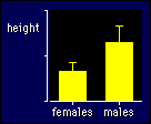
For example, if you are comparing females and males, check to see how different
the standard deviation is for the males vs the females (see the figure). Then,
if the sample size is the same in each group, forget about it! Yes, it doesn't
matter how different the standard deviations are, you get the right confidence
limits when the groups are the same size. But if the groups differ in size (e.g.,
by a factor of 1.1 or more) and the standard deviations differ too (also by
a factor of 1.1 or more), then you gotta do something. And the answer is...
use the t test with unequal variances! It would be better to call it
the t test with unequal standard deviations, but statisticians prefer to use
the term variance (the square of the standard deviation). Most stats
programs offer this option along with the usual t test. Your stats program may
even do an extra test of whether the variances within the two groups are equal,
but don't take any notice of the p value for that test. Look instead at the
size of the standard deviations and the sample sizes, then make your decision
about which form of the t test to use. Actually, when the variances are the
same and the sample sizes are the same, the confidence limits provided by the
two tests are practically identical, so you might as well always use the t test
with unequal variances
Uniformity of
Residuals in Complex Models
I have been dealing with uniformity of residuals
in simple models, which consist of one predictor
variable (height or sex in our examples). In more complex
models--those with two or more predictor variables--you should check the
uniformity of the residuals not just across the range of predicted values but
also across the range of values of each of the predictors. You do that by getting
your stats package to output all the residuals with corresponding values of
each predictor variable. For each predictor you then do a plot of the residuals
(Y axis) against the values of the predictor (X axis) and look for non-uniformity.
As in the first example above, you get a better idea of any non-uniformity
by plotting the mean and standard deviation of the residuals. For each nominal
predictor variable, you show the means and standard deviations on a single plot
that includes each level of the variable. For each numeric predictor, you group
the values of the predictor into quantiles of equal numbers of observations,
just like I explained above for the predicted values. You then plot the means
and standard deviations of the residuals against the mean of each quantile of
the predictor. Any consistent pattern in the mean of the residuals indicates
that the mathematical form of the model for that predictor is inadequate. For
example, you might need to introduce a quadratic or a non-linear term for that
variable into the model . Any substantial difference in the standard deviation
of the residuals for different levels or values of the predictor indicates that
you need to transform the dependent variable.
Go to: Next · Previous · Contents · Search
· Home
webmaster
Last updated 9 March 03
 It's easiest to understand
when the model you are fitting is a straight line. See the diagram, which is
the top corner of the height-weight graph blown up so you can see what's what.
The observed values are just the weights. The predicted values are the weights
on the line corresponding to each observed weight. You should be able to see
that if you drew a straight line further away from the points, the residuals
overall would get bigger.